参考网址

(116条消息) LQR 的直观推导及简单应用_白巧克力亦唯心的博客-CSDN博客_lqr算法

路径规划与轨迹跟踪系列算法学习_第12讲_线性二次型调节器(LQR)法_哔哩哔哩_bilibili

https://github.com/AtsushiSakai/PythonRobotics

解释

  • 对于一个线性系统可以用x_dot = Ax +Bu表示,参考全反馈控制模型,我们需要设计一个状态反馈控制器,表示为

    u = -Kx,使得闭环系统满足我们的期望性能.因此可以可得到状态方程为x_dot = (A-BK)x=Acx

1647741354_1_.png

  • 通过设计一款能量函数,如下,希望最优的控制轨迹应该使得该能量函数最小

20140914171220986.png

  • 由于u = -Kx,我们可以得到,

20140914171601165.png

  • 为便于求解K,引入常矩阵P,最终化简可以得到

1647742289_1_.png

  • lqr求解流程
    • 选择参数矩阵Q,R
    • 求解Riccati 方程得到矩阵P
    • 计算 : K = R*-1* BT P

lqr结构图

1647749530_1_.png

程序

倒立摆的状态变量为x=[p,p_dot,the,the_dot]T,其中p(t)是小车位置,θ是倒立摆的角度,这里直接调用matlab中lqr

1
2
3
4
5
6
7
8
9
10
11
12
13
14
15
16
17
18
19
20
21
22
23
A = [0 1 0 0
0 0 -1 0
0 0 0 1
0 0 9 0];
B = [0;0.1;0;-0.1];
C = [0 0 1 0]; %观测角度
D = 0;

Q = [1 0 0 0
0 1 0 0
0 0 10 0
0 0 0 10
];
R = 0.1;
%由上面这个系统,可以计算出K
K = lqr(A,B,Q,R);
Ac = A - B*K;
%对系统进行模拟
x0 = [0.1;0;0.1;0]; %初始状态
t = 0:0.05:20;
u = zeros(size(t));
[y,x]=lsim(Ac,B,C,D,u,t,x0);
plot(t,y);

python实现dlqr

1
2
3
4
5
6
7
8
9
10
11
12
13
14
15
16
17
18
19
20
21
22
23
24
25
26
27
28
29
30
31
32
def solve_DARE(A, B, Q, R):
"""
solve a discrete time_Algebraic Riccati equation (DARE)
"""
X = Q
maxiter = 150
eps = 0.01

for i in range(maxiter):
Xn = A.T @ X @ A - A.T @ X @ B @ \
la.inv(R + B.T @ X @ B) @ B.T @ X @ A + Q
if (abs(Xn - X)).max() < eps:
break
X = Xn
return Xn
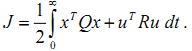
def dlqr(A, B, Q, R):
"""Solve the discrete time lqr controller.
x[k+1] = A x[k] + B u[k]
cost = sum x[k].T*Q*x[k] + u[k].T*R*u[k]
# ref Bertsekas, p.151
"""

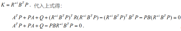
# first, try to solve the ricatti equation
X = solve_DARE(A, B, Q, R)

# compute the LQR gain
K = la.inv(B.T @ X @ B + R) @ (B.T @ X @ A)

eigVals, eigVecs = la.eig(A - B @ K)

return K, X, eigVals

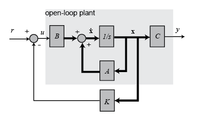
注意这里的A,B使用的是frenet坐标系

主要是[e,e_dot,the_e,the_e_dot]

关于加入纵向控制lqr算法

注意: x = [e, dot_e, th_e, dot_th_e, delta_v],当然相关的A,B,Q,R同样修改

1
2
3
4
5
6
7
8
9
10
11
12
13
14
15
16
17
18
19
20
21
22
23
24
25
26
27
28
29
30
31
32
33
34
35
36
37
38
39
40
41
42
43
44
45
46
47
48
49
50
51
52
53
54
55
56
57
58
59
60
61
62
def lqr_speed_steering_control(state, cx, cy, cyaw, ck, pe, pth_e, sp, Q, R):
ind, e = calc_nearest_index(state, cx, cy, cyaw)

tv = sp[ind]

k = ck[ind]
v = state.v
th_e = pi_2_pi(state.yaw - cyaw[ind])

# A = [1.0, dt, 0.0, 0.0, 0.0
# 0.0, 0.0, v, 0.0, 0.0]
# 0.0, 0.0, 1.0, dt, 0.0]
# 0.0, 0.0, 0.0, 0.0, 0.0]
# 0.0, 0.0, 0.0, 0.0, 1.0]
A = np.zeros((5, 5))
A[0, 0] = 1.0
A[0, 1] = dt
A[1, 2] = v
A[2, 2] = 1.0
A[2, 3] = dt
A[4, 4] = 1.0

# B = [0.0, 0.0
# 0.0, 0.0
# 0.0, 0.0
# v/L, 0.0
# 0.0, dt]
B = np.zeros((5, 2))
B[3, 0] = v / L
B[4, 1] = dt

K, _, _ = dlqr(A, B, Q, R)

# state vector
# x = [e, dot_e, th_e, dot_th_e, delta_v]
# e: lateral distance to the path
# dot_e: derivative of e
# th_e: angle difference to the path
# dot_th_e: derivative of th_e
# delta_v: difference between current speed and target speed
x = np.zeros((5, 1))
x[0, 0] = e
x[1, 0] = (e - pe) / dt
x[2, 0] = th_e
x[3, 0] = (th_e - pth_e) / dt
x[4, 0] = v - tv

# input vector
# u = [delta, accel]
# delta: steering angle
# accel: acceleration
ustar = -K @ x

# calc steering input
ff = math.atan2(L * k, 1) # feedforward steering angle
fb = pi_2_pi(ustar[0, 0]) # feedback steering angle
delta = ff + fb

# calc accel input
accel = ustar[1, 0]

return delta, ind, e, th_e, accel